Fine Margins

Let’s start by stating that Burnley are having an incredible Premier League campaign. Clarets boss Sean Dyche is notable for using his post-match interviews to point out that the club’s success has been decided by fine margins which is to say that many of their victories have been the result of outscoring the opposing team by a single goal.

Just how fine are the margins?

After hearing this sentiment echoed consistently by the manager, I had the idea to look at a metric for evaluating just how fine the margins have been. While all goals are valuable, the goal that makes the total scored one greater than the other team is the most valuable.

For people that don’t follow this sport, 3 points are awarded for a win and 1 point for a draw (As an American, saying the name of this sport is problematic and both options are sub-optimal). Goals above and beyond the goal needed to win have value in the event of a points tie at the end of the season as well as providing psychological and entertainment value however hopefully we can agree that the goal needed to win has the most value.

In some ways the metric we are building treats goals above and beyond the one needed to win as well as those scored in a loss as wasted effort. While not entirely true, for many teams it is critical to get as many points as possible from the relatively few goals they are able to score. With all this said, we can now somewhat easily calculate the point value of every goal to compare Burnley’s margins or maybe better yet their efficiency with the rest of the league.

Load the Data and Libraries

Football Data UK has an impressive amount of freely available data. We will load the results from the current Premier League season.

#libraries (we will do everything just using the tidyverse)
library(tidyverse)
 
# get data
epl <- read_csv("http://www.football-data.co.uk/mmz4281/1718/E0.csv")

## Warning: Missing column names filled in: 'X66' [66], 'X67' [67], 'X68' [68]

## Parsed with column specification:
## cols(
##   .default = col_double(),
##   Div = col_character(),
##   Date = col_character(),
##   HomeTeam = col_character(),
##   AwayTeam = col_character(),
##   FTHG = col_integer(),
##   FTAG = col_integer(),
##   FTR = col_character(),
##   HTHG = col_integer(),
##   HTAG = col_integer(),
##   HTR = col_character(),
##   Referee = col_character(),
##   HS = col_integer(),
##   AS = col_integer(),
##   HST = col_integer(),
##   AST = col_integer(),
##   HF = col_integer(),
##   AF = col_integer(),
##   HC = col_integer(),
##   AC = col_integer(),
##   HY = col_integer()
##   # ... with 9 more columns
## )

## See spec(...) for full column specifications.

Remove 0-0 draws

The objective of this exercise is to create a normalized value scale where the maximum value per goal would be 3 which is to say that a team wins every game by a score of 1-0. Given this, 0-0 draws need to be removed since these result in points being accumulated without goals being scored. If 0-0 draws were included then in theory a single goal could be valued at 40 points if 37 matches ended in 0-0 draws with just one 1-0 result.

# remove 0-0 draws by selecting only results where at least one team's goals are greater than 0
epl <- epl %>%
  filter(FTHG > 0 | FTAG > 0)

Stack the Results

Next, we will create summary tables for all possible results and stack these so we have one long dataset to use for plotting the value per goal metric.

home_wins <- epl %>%
  filter(FTR == "H") %>%
  select(HomeTeam, FTHG, FTR) %>%
  rename(team = HomeTeam, goals = FTHG) %>%
  mutate(points = 3)
 
home_loss <- epl %>%
  filter(FTR == "A") %>%
  select(HomeTeam, FTHG, FTR) %>%
  rename(team = HomeTeam, goals = FTHG) %>%
  mutate(points = 0)
 
away_wins <- epl %>%
  filter(FTR == "A") %>%
  select(AwayTeam, FTAG, FTR) %>%
  rename(team = AwayTeam, goals = FTAG) %>%
  mutate(points = 3)
 
away_loss <- epl %>%
  filter(FTR == "H") %>%
  select(AwayTeam, FTAG, FTR) %>%
  rename(team = AwayTeam, goals = FTAG) %>%
  mutate(points = 0)
 
home_draws <- epl %>%
  filter(FTR == "D") %>%
  select(HomeTeam, FTHG, FTR) %>%
  rename(team = HomeTeam, goals = FTHG) %>%
  mutate(points = 1)
 
away_draws <- epl %>%
  filter(FTR == "D") %>%
  select(AwayTeam, FTAG, FTR) %>%
  rename(team = AwayTeam, goals = FTAG) %>%
  mutate(points = 1)
 
goals_to_points <- bind_rows(
  home_wins, 
  home_loss, 
  away_wins, 
  away_loss, 
  home_draws, 
  away_draws
  )

Plotting the Metric

Lastly, we can plot our newly created metric using the proper club colors of course (thanks to: Jim Nielsen)

goals_to_points %>%
  group_by(team) %>%
  summarise(goals = sum(goals), points = sum(points), goal_point_value = points/goals) %>%
  mutate(team = fct_reorder(team, goal_point_value)) %>%
  ggplot(aes(y = goal_point_value, x = team, fill = team)) +
  geom_col() +
  coord_flip() +
  theme(panel.background = element_blank(), 
        panel.grid.major.y = element_line(color = "light grey", size = 0.25), 
        legend.position="none") +
  scale_fill_manual(values = c("#091453","#F7C240","#ED1A3B","#00A398","#EF0107","#0053A0","#E03A3E","#FBEE23","#1B458F","#E62333","#98C5E9","#001C58","#DBA111","#274488","#241F20","#F8BC1B","#0073D2","#000000","#DA020E","#8CCCE5")) + 
  labs(x = NULL, y = NULL, title = "Premier League Point Value Per Goal")

Dizzying Heights

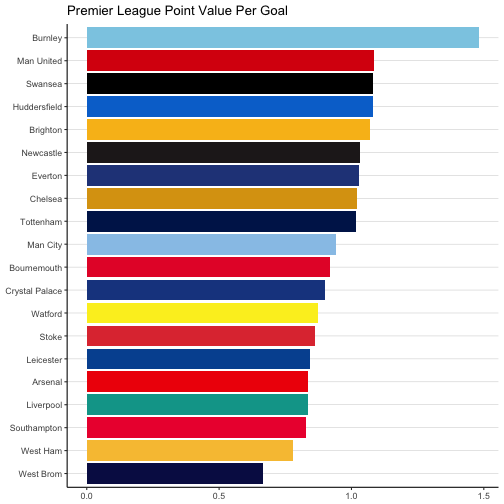
Without the ability to pay the salaries that other teams pay, Burnley need to be as efficient as possible. Our plot shows that they have, in fact, far outpaced the rest of the league in value per goal. At one point in the season, Burnley were as high as fourth in the league table – a position described as “dizzying heights” by many pundits. However, as of this post, Burnley have a real chance to finish in the Top 6 – a segment of the league usually reserved for the same six teams every year.

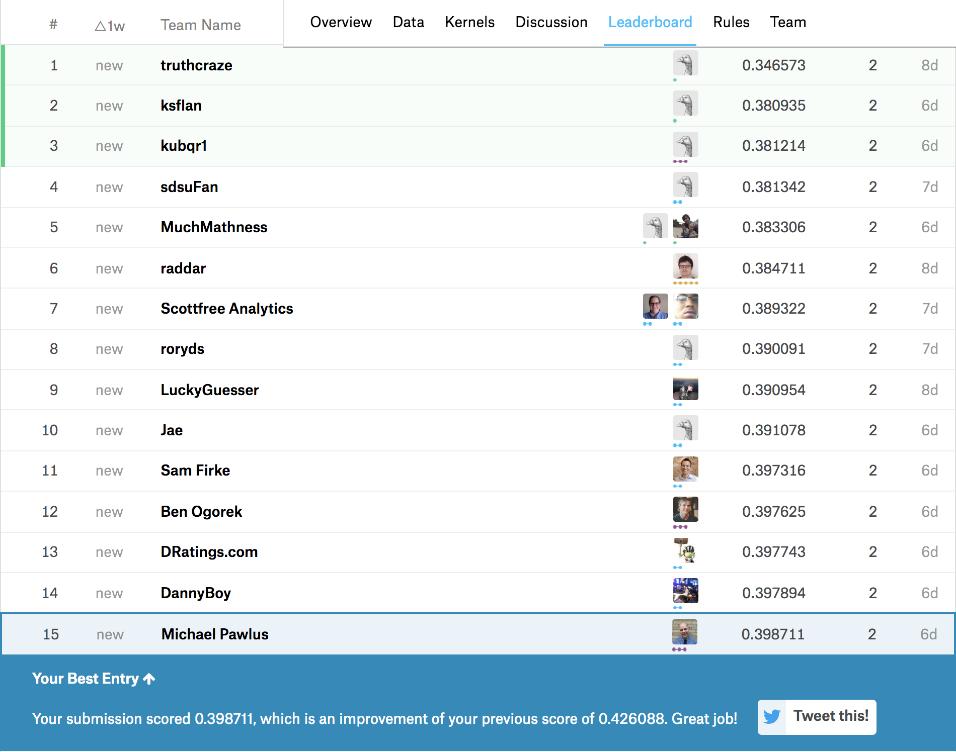
Also, as of this post, I am 15th in a Kaggle competition and I think there is a real chance I can finish Top 3 for the first time ever.

Where will Burnley and I land? We will know before long…